Detecting distribution changes in data streams

$\require{textcomp}$Many real world problems involve time component, which describes some phenomenon that that evolves over time. Examples could include network traffic monitoring, video survelliance, machinery vibration status and many more.

This evolution over time generally implies the concept of data stream, according to which, data points are observed sequentially and over time, rather than all at once.

During such observation, the data stream could start manifesting some changes that might be relevant to our use-case (e.g. a sudden change in network traffic, abnormal video surveillance activity, change in usual user’s behaviour, etc.) and that we might be interested in detecting.

Task

Given data stream setting, we would like to have a model learn the dynamics of the incoming data, and be able to detect whether or not a change has occurred in the data generating distribution. Such a change could be due to changes in underlying both function and/or parameters.

Areas highlighted by red indicate changes in stream distribution.

More formally:

• Suppose we are observing a random process $P$ that at each time step emits a value sampled from a probability distribution $\mathcal{P}(\bar{\theta}_1)$ where $\bar{\theta}_1$ is a set of parameters for the distribution.

• Suppose that at some point in time, $t’$ the process $P$ is subject to a change in the underlying data distribution to $\mathcal{D}(\bar{\theta}_2)$.

• Our task would be thus that of detecting the time of change $t’$ as quicky as possible.

Approach

In this post we will present one possible approach to automatically detect such changes, that is based on martingale testing, defined in A Martingale Framework for Detecting Changes in Data Streams by Testing Exchangeability [1].

In a nutshell, the idea is the following:

• This algorithm keeps a set of points captured online, updated on arrival.

• A statistical test is used to estimate the likelihood of the new point to follow the distribution of the captured set of points.

• As the stream starts shifting in distribution, the likelihood of the new points to follow the online set distribution will become lower over time.

• Once enough evidence has been accumulated against the “all captured points belong to same distribution” hypothesis, a condition is triggered to detect the change in distribution.

Building blocks of the algorithm

• Strangeness function: a function that given a set of points $T=\{x_1,…,x_n\}$, computes how much an incoming data point $x$ is different from the other data points in the set $T$. One example of a strangeness function could is the clustering strangeness $f(T, x) = \left\lVert x - \text{centroid}(T) \right\rVert$.

• Martingale: intuitively, a martingale is a sequence of random variables that remains stable in value with some fluctuations as long as the process is random (at any particular time, the conditional expectation of the next value in the sequence is equal to the present value, regardless of all prior values).

• Exchangeability property: a sequence of random variables $Z_1, …, Z_n$ is said to be exchangeable iff $P(Z_1, …, Z_n) = P(Z_{\pi(1)}, …, Z_{\pi(n)})$ where $\pi$ is a permutation function (the sequence is invariant under any permutation of its indices).

• Exchangeability null hypothesis: the algorithm operates under a null hypothesis $H_0$ that the date sequence is exchangeable (i.e. exchangeability property holds).

Algorithm sketch

1. A set of data points, called “current set” is used to store all the points that are being used for distribution shift detection, this set will be updated online.
2. Once a new point is observed, its strangeness (e.g. cluster strangeness) with the data points in current set will be computed, measuring how different is this new point from the current set of points (the centroid they form).
3. Additionally, the algorithm computes the randomized power martingale value reflecting the strength of evidence found against the null hypothesis of data exchangeability property.
4. Randomized power martingale is defined as $M_n^{(\epsilon)} = \prod_{i=1}^n \epsilon\hat{p}_i^{\epsilon - 1}$ where $\hat{p}$ is called $\hat{p}$-value function, such that $\hat{p}({x_1,…,x_i}, \theta_i) = \frac{| \{ j:s_j>s_i \} | + \theta_i | \{ j:s_j=s_i \} |}{i}$ with $\theta_i \sim U(0, 1)$.
5. If points are generated from a source that satisfies exchangeability property (i.e. points are coming from the same distribution), then there’s a property that $\hat{p}$-values will be distributed uniformly on $[0, 1]$. However, if this property is violated, then $\hat{p}$-values will no longer be distributed uniformly in $[0, 1]$ (due to strangeness of newer points being likely higher), as a result $M_n^{(\epsilon)}$ will increase, providing more evidence against null hypothesis $H_0$ of sequence exchangeability. The algorithm employs this property of $M_n^{(\epsilon)}$ to aid with detecting changes.
6. Martingale test continues to operate as long as $0 \lt M_n^{(\epsilon)} \lt \lambda$, and the null hypothesis $H_0$ is rejected when $M_n^{(\epsilon)} \geq \lambda$ (i.e. “no change in data stream” hypothesis has a high evidence against it).
7. The parameter $\lambda$ indicates a degree of false alarm rate (FAR) we are willing to accept from our detector.

Experiments

The remaining structure of this post will report experiment results on the following two scenarios:

1. Synthetic example: example of applying the detector on an easy synthetic dataset.
2. Real world example: example of applying the detector on a more complicated, real-world dataset representing accelerometer signals of a machinery in which a pump cavitation was induced, making the machinery fail.

To follow along, please run the notebook from this project’s repository as specified in the instructions.

Synthetic example

In order to test the algorithm implementation, we start by applying it to a synthetically generated data stream.

The advantage of synthetic data is that we can control the way it is generated in order to challenge our algorithm and find bugs, if present.

In the previously mentioned repository, we’ve implemented a synthetic data generation procedure that given:

1. A list of means $\mu_1,…,\mu_K$
2. A list of standard deviations $\sigma_1,…,\sigma_K$
3. A list of durations $d_1,…,d_K$

outputs a signal where i-th interval would contain $d_i$ samples taken from $\mathcal{N}(\mu_i, \sigma_i)$, for i $\in {1,..,K}$

To generate a synthetic signal we can run the following:

# Define parameters of synthetic data
sizes_synthetic = [600, 500, 1050, 500]
means_synthetic = [0.34, 1.5, 2.9, 1.5]
std_synthetic = 0.8
changes_gt_synthetic = np.cumsum(sizes_synthetic)[:-1]
# Generate synthetic timeseries dataset
data_synthetic = generate_synthetic_normal(
    locs=means_synthetic, 
    sizes=sizes_synthetic, 
    scale=std_synthetic, dims=1
)
data_df_synthetic = pd.DataFrame(data_synthetic)

Visually we can plot it and have changes of distribution highlighted by a different shade of red:

plot_total_df(
    data_df_synthetic, 
    "Signal", 
    changes=changes_gt_synthetic, 
    max_intensity=0.6
)

Let us now run the previously described Martingale Test algorithm on our synthetic dataset:

martingale_tester_synthetic = MartingaleTest(2, epsilon=0.96)
changes_pred_synthetic = run_martingale_tester(
    martingale_tester_synthetic,
    data_synthetic
)

plot_total_df(
    data_df_synthetic, 
    "Signal", 
    changes=changes_pred_synthetic,
    gt_changes=changes_gt_synthetic,
    max_intensity=0.6,
)

And view the results, where the green lines indicate groundtruth distribution change times and areas highlighted by shades of red indicate changes in stream distribution detected by martingale tester:

In terms of metrics, we can measure precision, recall and F1 for a window of K timesteps around the groundtruth values.

For example, with K=75, the previous result yields the following metrics.

Precision: 0.75
Recall: 1.0
F1: 0.86

Right out of the box we’ve managed to obtain a recall of 1.0, as can be confirmed by the plot, however the precision seems to be a little off. Overall we can say we’re satisfied with the recall and don’t need to perform a hyperparameter search.

Real World Example

Let us now try to run the approach on a real world dataset.

The dataset contains 6 signals, x,y,z measurements of two accelerometers with an induced cavitation phenomenon, with data spread over several files.

For simplicity reasons, data in our repository was already preprocessed, producing a single dataframe with relative streams identified by a special field. Additionally 75000 samples per time unit were aggregated into single samples by their statistics: mean, stddev, skewness, kurtosis.

The final preprocessed version is included in the repository and has the following structure:

Time	P1_x	P1_y	P1_z	P2_x	P2_y	P2_z	stream_id	status
2013-01-10 08:28:35.281	-0.018477	-0.007019	0.001150	0.046848	0.031780	0.050179	0	0
2013-01-10 08:28:38.281	-0.018573	-0.007016	0.000854	0.046712	0.031624	0.049469	0	0
…	…	…	…	…	…	…	…	…

Visualizing it, yields the following plots with distribution change indicated by a shade of red:

For a simpler visualization, we can also average across all the 6 signals to produce a single signal which more or less maintains the properties of the original signals:

Distribution drift detection

Let us now apply our martingale testing technique to detect changes of distribution.

martingale_tester = MartingaleTest(6, epsilon=0.80)

series_np = np.concatenate((
    statistical_features_averaged_train["mean"]["average_column"].to_numpy().reshape(-1, 1),
    statistical_features_averaged_train["std"]["average_column"].to_numpy().reshape(-1, 1),
    statistical_features_averaged_train["skewness"]["average_column"].to_numpy().reshape(-1, 1),
    statistical_features_averaged_train["kurtosis"]["average_column"].to_numpy().reshape(-1, 1),
    ), axis=-1
)
changes_pred = run_martingale_tester(
    martingale_tester,
    series_np
)

metrics_in_range(gt=changes_gt, pred=changes_pred, interval=20)

{'precision': 0.20833333333333334,
 'recall': 0.8333333333333334,
 'F1': 0.33333333333333337}

Despite having a high recall, we observe a low precision, this comes from the fact that the algorithm might be very sensitive to distribution changes, generating a high number of false alarms.

Let us see if we can find a combination of tester parameters that can give better results in terms of precision and F1:

# grid search
epsilon = [0.80, 0.81, 0.82, 0.83, 0.84, 0.85, 0.86, 0.87, 0.88, 0.89, 0.9, 0.91, 0.92, 0.93, 0.94, 0.95, 0.96, 0.97, 0.98, 0.99]
M = [4, 5, 6, 7, 8, 9, 10, 11, 12, 13, 14, 15, 16, 17, 18, 19, 20]
# interval window inside which we consider a predicted change to hold true
# note that 1 unit of interval corresponds to 3 seconds of real time.
interval = 20
best_params, out_lists = martingale_tester_grid_search(series_np, changes_gt, epsilon, M, interval, verbose=0)

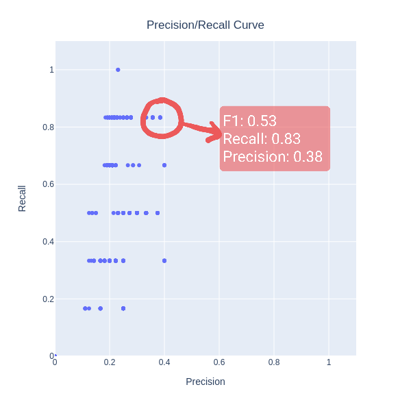
Grid search results visualized in terms of precision-recall scatter plot. Notice that here we aren't looking for a classification threshold, but rather just trying to visualize what is the recall we can give away to obtain better precision.

From the plot we can see what are our trade-off options between precision and recall.

Best parameters found by the grid search yield the following metrics:

{'F1': 0.5263157894736842,
 'params': (0.89, 20),
 'recall': 0.8333333333333334,
 'precision': 0.38461538461538464}

best_martingale_tester = MartingaleTest(best_params["params"][1], epsilon=best_params["params"][0])

changes_pred = run_martingale_tester(
    best_martingale_tester,
    series_np
)

changes_gt_indexes = statistical_features_averaged_train["kurtosis"]["average_column"].index[changes_gt]

plot_total_df(
    statistical_features_averaged_train["kurtosis"]["average_column"], 
    "Kurtosis", 
    changes=changes_pred,
    gt_changes=changes_gt_indexes,
    max_intensity=0.8
)

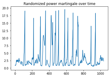
We can also visualize the accumulated martingale values over time, this allows us to see what were the points in which algorithm made the decisions to detect change of distribution:

Conclusions

• The Martingale Tester algorithm is a very simple and intuitive algorithm.

• When the distribution changes are “simple”, such as in the case of synthetic data, the algorithm can perform well even out of the box.

• When the signal instead is more complicated, as observed in real world dataset section, the algorithm might have difficulties with maintaining a high precision, due to a relativly high false alarm rate, despite being ran with a more optimal set of parameters.

• In order to work well with such data, more powerful and modern approaches should be used.

References

[1] S. Ho and H. Wechsler, “A Martingale Framework for Detecting Changes in Data Streams by Testing Exchangeability,” in IEEE Transactions on Pattern Analysis and Machine Intelligence, vol. 32, no. 12, pp. 2113-2127, Dec. 2010, doi: 10.1109/TPAMI.2010.48.